Markov Decision Processes: Formulating the Best Possible Decisions
by Veronica Scerra
A ground-up exploration of Reinforcement Learning methods and models.
Reinforcement learning is the science of learning to make decisions, or conversely, teaching machines to make decisions based on environmental variables. In our discussion of k-armed bandits, I introduced the idea of actions - multiple actions that can be taken in a situation, but the model in that situation is one of actions and rewards. This brings us to Markov Decision Processes (MDPs), which formalize the problem with a full sequential structure. If we assume that the environment is fully observable, and we also assume that the current observation contains all of the relevant information for understanding our state and options, then we can create a model of best choices in our current state for maximum reward. In an MDP, actions not only influence immediate rewards, but also future rewards through subsequent situations and states, all of which are, or can be, known. In the bandit problem, we estimated the value of each action taken, in MDPs, we extend that to estimate the value of each action in each state, or we estimate the value of each state given optimal action selections. In the model for a MDP, the learner or decision maker is called the agent, and the things the agent interacts with are the environment.
The Key Players in an MDP
The key elements that comprise an MDP model are as follows:
- State (S) : "Where am I?"
- Represents the situation the agent is in at a given time point (t)
- Can be physical locations (e.g., grid positions), system status (e.g., health levels), or abstract configurations
- The agent starts in some state \( s ∈ S \)
- Actions (A) : "What can I do?"
- A set of choices available to the agent in any given state
- Denoted as \( a(s) \): actions available in state \( s \)
- The agent selects an action \( a ∈ A(s) \) to try and maximize its future reward
- Transition Probabilities (P) : "What happens if I act?"
- Define the dynamics of the environment: \( P(s'|s, a) \) = Probability of ending in state \( s' \) after taking action \( a \) in state \( s \)
- The probability used in this formulation captures stochasticity - the same action may not always lead to the same outcome.
- Interaction: Given a current state \( s \) and a chosen action \( a \), the environment uses \( P \) to select the next state \( s' \)
- Reward Function (R) : "What do I get?"
- Tells the agent how good it is to take action \( a \) in state \( s \) and land in state \( s' \)
- \( R(s, a, s') \): reward for transitioning from state \( s \) to \( s' \) via \( a \)
- Simplified as \( R(s, a) \) or \( R(s') \), depending on the context
- Interaction: When the agent transitions from \( s \) → \( s' \) via \( a \), the reward is given immediately \(r = R(s, a, s') \)
- Discount Factor (γ) : "How much do I care about the future?"
- A scalar in [0, 1) that determines how future rewards are weighted
- γ ≈ 0: agent prefers immediate rewards ("short-sighted")
- γ ≈ 1: agent values long-term rewards ("far-sighted")
- Interaction: Used when computing cumulative rewards
\[ G_{t} = R_{t+1} + γR_{t+2} + γ^{2}R_{t+3} + … = \sum_{k=0}^{∞} γ^{k} R_{t+k+1} \]
Where t represents the time step and γ is the discount factor
Typical Formulation:
Putting it All Together: The Agent-Environment Loop
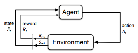
Depiction of the agent-environment interactions in a MDP, borrowed from Sutton & Barto (2018)
At each timestep \(t\)
- Agent observes the current state \(S_{t}\)
- Agent chooses action \(A_{t}\)
- Environment samples the next state \(S_{t+1}\)
- Environment provides reward \(R_{t+1} = R(S_{t}, A_{t}, S_{t+1})\)
- Agent updates its value estimates or policy using \((S_{t}, A_{t}, R_{t+1}, S_{t+1})\)
- Repeat …
In a finite MDP, the sets of states, actions, and rewards all have a finite number of elements (as opposed to infinite…)
Agent's Learning Objectives: What's the Point?
To what end are we specifying all of these key players and parameterizing the learning system? What does all of this accomplish?
Goals: In an MDP, the agent’s goal is to find a way to act (a policy) that maximizes cumulative reward over time. Crucially, the goal isn’t to get the biggest reward at one time step, but rather to develop a reliable strategy for maximizing total expected reward over time. This is a long-term goal that incorporates discount factors for distal vs. proximal rewards, many time steps, and reliable reward expectations.
Specifying rewards carefully is crucial to developing a winning strategy for maximizing reward. For example, if you were teaching an agent to navigate a maze, you would give positive rewards for reaching the end and penalize time spent in the maze to encourage the agent to complete the maze as quickly as possible. If you wanted a robot to learn how to walk, you would positively reward forward motion, and negatively reward stumbles, falls, and instability - the machine would soon learn to stabilize and move forward to avoid the negative rewards and maximize the returns for the episode of walking. In these instances, in this problem formulation for reinforcement learning, the “purpose” or “goal” can be thought of as the maximization of the expected value of a cumulative return value, also called reward.
Policy: The policy adopted by an agent answers the question “What should I do to maximize reward?” What I personally find fascinating about reinforcement learning is that it really is just a formalization of what humans (and all animals) do naturally. You observe patterns, you formulate a plan for getting the most reward (often, you don’t even do it consciously), and you continually evaluate your returns and adjust your approach. That plan you formulate for getting the best coffee by standardizing your order, finding the best grocery store by evaluating the pros and cons of getting there/selection/prices/ convenience, or choosing which of your neighbors you like best are all examples of adopting a policy for maximizing returns. Our determination of “good” actions to take is usually based on our expected reward policy.
Formally, policy is a mapping from states to probabilities of selecting each possible action. The ultimate goal of reinforcement learning is to find the optimal policy, denoted \(π^{*}\). The policy is defined to answer the question - “Given that I’m in state , what action should I take?” Policies can come in two flavors: deterministic and stochastic.
- Deterministic Policy: \(π(s)\) → always take action \(a\) in state \(s\)
- Stochastic Policy: \(π(a|s)\) → assigns a probability to taking action \(a\) in state \(s\)
Value Function: The value function is the formalization assigning expected return to states and actions. It answers the question - “How good is this action/state?” in the context of possibilities available. Value functions can be assigned to both states and actions as follows:
- State value function (\(V^{π}(s)\))
"Given the state \(s\), the expected reward will be the following, assuming we take the subsequent actions dictated under our policy \(π\)" \[ V^{\pi}(s) = \mathbb{E}_{\pi} \left[ \sum_{t=0}^{\infty} \gamma^t R_{t+1} \,\middle|\, S_0 = s \right] \]
- Action value function (\(Q^{π}(s,a)\))
"Given the state \(s\) and action \(a\), the expected reward will be the following, assuming we take the subsequent actions dictated under our policy \(π\)" \[ Q^{\pi}(s, a) = \mathbb{E}_{\pi} \left[ \sum_{t=0}^{\infty} \gamma^t R_{t+1} \,\middle|\, S_0 = s, A_0 = a \right] \]
Once your value functions are specified, it is simple work to select the best action/state combination for your policy to maximize returns
Putting it All Together: Goals, Policies, and Value Functions
- Goals interact with all other elements to find the best policy \(π^{*}\) to maximize expected reward. Goal = “let’s get the best return possible”
- Policy can be either deterministic or stochastic, and the decision for what to is enacted by adopting value functions to maximize returns. Policy = “We can get the best return by making the following choices..."
- Value functions guide the policy to estimate anticipated return assuming the current policy is followed. Value function = “These are the expected rewards for making these choices in our current state”
- Feedback loop: Update policy based on value estimates → update value estimates based on new policy (e.g., in policy iteration).
The truly cool thing about a finite MDP is that all of the actions, states, and rewards can be known, so that in any situation a policy and value functions can be specified and the best path forward to maximize reward can be chosen. Next post will address the Bellman Equation, which ties all of the elements together mathematically.
Visual Insights and Experimental Notebook
The notebook that corresponds with this post (found here) illustrates:
- How states and actions affect transitions
- Reward dynamics and terminations
- Stochastic transitions in action
- Visual representations of policy and value iteration
This work lays the foundation for more complex reinforcement learning problems like multi-step decision making, function approximation, and dynamic environments.
What's Next?
Now that we understand the elements contributing to MDPs, I plan to expand this series into:
- Non-stationary bandits with decaying reward probabilities
- Contextual bandits, incorporating features for smarter decision making
- Q-learning and SARSA algorithms
- Deep Reinforcement Learning using neural networks to approximate value functions (the good stuff)
This ongoing series project aims to demystify reinforcement learning concepts through hands-on code, clear explanations, and visualizations. Learn with me!